Something More for Research

Explorer of Research #HEMBAD

Tutorials for Deep Learning

Posted by Hemprasad Y. Badgujar on September 8, 2016


  1. UFLDL: http://deeplearning.stanford.edu/wiki/index.php/UFLDL_Tutorial
  2. CS231n@Standford: http://cs231n.stanford.edu/syllabus.html
  3. DL Summer School 2015:https://sites.google.com/site/deeplearningsummerschool/schedule
  4. BIL 722@Hacettepe University:http://web.cs.hacettepe.edu.tr/~aykut/classes/spring2016/bil722/
  5. CSC2523@University of Toronto:http://www.cs.utoronto.ca/~fidler/teaching/2015/CSC2523.html
  6. CSC321@University of Toronto: http://www.cs.toronto.edu/~tijmen/csc321/
  7. DL@New York University: http://cilvr.cs.nyu.edu/doku.php?id=deeplearning:slides:start
  8. ECE 6504@Virginia Tech: https://computing.ece.vt.edu/~f15ece6504
  9. ML@Oxford University: https://www.cs.ox.ac.uk/people/nando.defreitas/machinelearning/
  10. DL Book (MIT Press): http://www.deeplearningbook.org/
  11. Ultimate resource page: http://www.jeremydjacksonphd.com/category/deep-learning/

Posted in Mixed | Leave a Comment »

Deep Learning Software/ Framework links

Posted by Hemprasad Y. Badgujar on July 15, 2016


  1. Theano – CPU/GPU symbolic expression compiler in python (from MILA lab at University of Montreal)
  2. Torch – provides a Matlab-like environment for state-of-the-art machine learning algorithms in lua (from Ronan Collobert, Clement Farabet and Koray Kavukcuoglu)
  3. Pylearn2 – Pylearn2 is a library designed to make machine learning research easy.
  4. Blocks – A Theano framework for training neural networks
  5. Tensorflow – TensorFlow™ is an open source software library for numerical computation using data flow graphs.
  6. MXNet – MXNet is a deep learning framework designed for both efficiency and flexibility.
  7. Caffe -Caffe is a deep learning framework made with expression, speed, and modularity in mind.Caffe is a deep learning framework made with expression, speed, and modularity in mind.
  8. Lasagne – Lasagne is a lightweight library to build and train neural networks in Theano.
  9. Keras– A theano based deep learning library.
  10. Deep Learning Tutorials – examples of how to do Deep Learning with Theano (from LISA lab at University of Montreal)
  11. Chainer – A GPU based Neural Network Framework
  12. DeepLearnToolbox – A Matlab toolbox for Deep Learning (from Rasmus Berg Palm)
  13. Cuda-Convnet – A fast C++/CUDA implementation of convolutional (or more generally, feed-forward) neural networks. It can model arbitrary layer connectivity and network depth. Any directed acyclic graph of layers will do. Training is done using the back-propagation algorithm.
  14. Deep Belief Networks. Matlab code for learning Deep Belief Networks (from Ruslan Salakhutdinov).
  15. RNNLM– Tomas Mikolov’s Recurrent Neural Network based Language models Toolkit.
  16. RNNLIB-RNNLIB is a recurrent neural network library for sequence learning problems. Applicable to most types of spatiotemporal data, it has proven particularly effective for speech and handwriting recognition.
  17. matrbm. Simplified version of Ruslan Salakhutdinov’s code, by Andrej Karpathy (Matlab).
  18. deeplearning4j– Deeplearning4J is an Apache 2.0-licensed, open-source, distributed neural net library written in Java and Scala.
  19. Estimating Partition Functions of RBM’s. Matlab code for estimating partition functions of Restricted Boltzmann Machines using Annealed Importance Sampling (from Ruslan Salakhutdinov).
  20. Learning Deep Boltzmann Machines Matlab code for training and fine-tuning Deep Boltzmann Machines (from Ruslan Salakhutdinov).
  21. The LUSH programming language and development environment, which is used @ NYU for deep convolutional networks
  22. Eblearn.lsh is a LUSH-based machine learning library for doing Energy-Based Learning. It includes code for “Predictive Sparse Decomposition” and other sparse auto-encoder methods for unsupervised learning. Koray Kavukcuoglu provides Eblearn code for several deep learning papers on thispage.
  23. deepmat– Deepmat, Matlab based deep learning algorithms.
  24. MShadow – MShadow is a lightweight CPU/GPU Matrix/Tensor Template Library in C++/CUDA. The goal of mshadow is to support efficient, device invariant and simple tensor library for machine learning project that aims for both simplicity and performance. Supports CPU/GPU/Multi-GPU and distributed system.
  25. CXXNET – CXXNET is fast, concise, distributed deep learning framework based on MShadow. It is a lightweight and easy extensible C++/CUDA neural network toolkit with friendly Python/Matlab interface for training and prediction.
  26. Nengo-Nengo is a graphical and scripting based software package for simulating large-scale neural systems.
  27. Eblearn is a C++ machine learning library with a BSD license for energy-based learning, convolutional networks, vision/recognition applications, etc. EBLearn is primarily maintained by Pierre Sermanet at NYU.
  28. cudamat is a GPU-based matrix library for Python. Example code for training Neural Networks and Restricted Boltzmann Machines is included.
  29. Gnumpy is a Python module that interfaces in a way almost identical to numpy, but does its computations on your computer’s GPU. It runs on top of cudamat.
  30. The CUV Library (github link) is a C++ framework with python bindings for easy use of Nvidia CUDA functions on matrices. It contains an RBM implementation, as well as annealed importance sampling code and code to calculate the partition function exactly (from AIS lab at University of Bonn).
  31. 3-way factored RBM and mcRBM is python code calling CUDAMat to train models of natural images (from Marc’Aurelio Ranzato).
  32. Matlab code for training conditional RBMs/DBNs and factored conditional RBMs (from Graham Taylor).
  33. mPoT is python code using CUDAMat and gnumpy to train models of natural images (from Marc’Aurelio Ranzato).
  34. neuralnetworks is a java based gpu library for deep learning algorithms.
  35. ConvNet is a matlab based convolutional neural network toolbox.
  36. Elektronn is a deep learning toolkit that makes powerful neural networks accessible to scientists outside the machine learning community.
  37. OpenNN is an open source class library written in C++ programming language which implements neural networks, a main area of deep learning research.
  38. NeuralDesigner  is an innovative deep learning tool for predictive analytics.
  39. Theano Generalized Hebbian Learning.

Posted in C, Computing Technology, CUDA, Deep Learning, GPU (CUDA), JAVA, OpenCL, PARALLEL, PHP, Project Related | Leave a Comment »

OpenCV 3.1 with CUDA , QT , Python Complete Installation on Windows in With Extra Modules

Posted by Hemprasad Y. Badgujar on May 13, 2016


OpenCV 3.1 with CUDA , QT , Python Complete Installation on Windows in With Extra Modules

The description here was tested on Windows 8.1 Pro. Nevertheless, it should also work on any other relatively modern version of Windows OS. If you encounter errors after following the steps described below, feel free to contact me.

Note :  To use the OpenCV library you have two options: Installation by Using the Pre-built Libraries or Installation by Making Your Own Libraries from the Source Files. While the first one is easier to complete, it only works if you are coding with the latest Microsoft Visual Studio IDE and doesn’t take advantage of the most advanced technologies we integrate into our library.

I am going to skip Installation by Using the Pre-built Libraries is it is easier to install even for New User. So Let’s Work on Installation by Making Your Own Libraries from the Source Files (If you are building your own libraries you can take the source files from OpenCV Git repository.) Building the OpenCV library from scratch requires a couple of tools installed beforehand

Prerequisites  Tools

Step By Step Prerequisites Setup

  • IDE : Microsoft Visual Studio. However, you can use any other IDE that has a valid CC++ compiler.

    Installing By Downloading from the Product Website Start installing Visual Studio by going to Visual Studio Downloads on the MSDN website and then choosing the edition you want to download.here we will going to use Visual Studio 2012 / ISO keys with  Visual Studio 2012 Update 4 /ISO and Step By Step Installing Visual Studio Professional 2012
  • Make Tool : Cmake is a cross-platform, open-source build system.

    Download and install the latest stable binary version: here we will going to use CMake 3 Choose the windows installer (cmake-x.y.z-win32.exe) and install it. Letting the cmake installer add itself to your path will make it easier but is not required.

  • Download OpenCV source Files by GIT/Sourceforge by : TortoiseGit or download source files from page on Sourceforge.

    The Open Source Computer Vision Library has >2500 algorithms, extensive documentation and sample code for real-time computer vision. It works on Windows, Linux, Mac OS X, Android and iOS.

  •  Python and Python libraries : Installation notes

    • It is recommended to uninstall any other Python distribution before installing Python(x,y)
    • You may update your Python(x,y) installation via individual package installers which are updated more frequently — see the plugins page
    • Please use the Issues page to request new features or report unknown bugs
    • Python(x,y) can be easily extended with other Python libraries because Python(x,y) is compatible with all Python modules installers: distutils installers (.exe), Python eggs (.egg), and all other NSIS (.exe) or MSI (.msi) setups which were built for Python 2.7 official distribution – see the plugins page for customizing options
    • Another Python(x,y) exclusive feature: all packages are optional (i.e. install only what you need)
    • Basemap users (data plotting on map projections): please see the AdditionalPlugins
  • Sphinx is a python documentation generator

    After installation, you better add the Python executable directories to the environment variable PATH in order to run Python and package commands such as sphinx-build easily from the Command Prompt.

    1. Right-click the “My Computer” icon and choose “Properties”

    2. Click the “Environment Variables” button under the “Advanced” tab

    3. If “Path” (or “PATH”) is already an entry in the “System variables” list, edit it. If it is not present, add a new variable called “PATH”.

      • Right-click the “My Computer” icon and choose “Properties”

      • Click the “Environment Variables” button under the “Advanced” tab

      • If “Path” (or “PATH”) is already an entry in the “System variables” list, edit it. If it is not present, add a new variable called “PATH”.

      • Add these paths, separating entries by ”;”:

        • C:\Python27 – this folder contains the main Python executable
        • C:\Python27\Scripts – this folder will contain executables added by Python packages installed with pip (see below)

        This is for Python 2.7. If you use another version of Python or installed to a non-default location, change the digits “27” accordingly.

      • Now run the Command Prompt. After command prompt window appear, type python and Enter. If the Python installation was successful, the installed Python version is printed, and you are greeted by the prompt>>> . TypeCtrl+Z and Enter to quit.

        Add these paths, separating entries by ”;”:

        • C:\Python27 – this folder contains the main Python executable
        • C:\Python27\Scripts – this folder will contain executables added by Python packages installed with easy_install (see below)

        This is for Python 2.7. If you use another version of Python or installed to a non-default location, change the digits “27” accordingly.

        After installation, you better add the Python executable directories to the environment variable PATH in order to run Python and package commands such as sphinx-build easily from the Command Prompt.

      • Install the pip command

      Python has a very useful pip command which can download and install 3rd-party libraries with a single command. This is provided by the Python Packaging Authority(PyPA): https://groups.google.com/forum/#!forum/pypa-dev

      To install pip, download https://bootstrap.pypa.io/get-pip.py and save it somewhere. After download, invoke the command prompt, go to the directory with get-pip.py and run this command:

      C:\> python get-pip.py
      

      Now pip command is installed. From there we can go to the Sphinx install.

      Note :pip has been contained in the Python official installation after version

        of Python-3.4.0 or Python-2.7.9.
  • Installing Sphinx with pip

    If you finished the installation of pip, type this line in the command prompt:

    C:\> pip install sphinx
    

    After installation, type sphinx-build -h on the command prompt. If everything worked fine, you will get a Sphinx version number and a list of options for this command.

    That it. Installation is over. Head to First Steps with Sphinx to make a Sphinx project.

    Now run the Command Prompt. After command prompt window appear, type python and Enter. If the Python installation was successful, the installed Python version is printed, and you are greeted by the prompt>>> . TypeCtrl+Z and Enter to quit.

  • Install the easy_install command

    Python has a very useful easy_install command which can download and install 3rd-party libraries with a single command. This is provided by the “setuptools” project: https://pypi.python.org/pypi/setuptools.

    To install setuptools, download https://bitbucket.org/pypa/setuptools/raw/bootstrap/ez_setup.py and save it somewhere. After download, invoke the command prompt, go to the directory with ez_setup.py and run this command:

    C:\> python ez_setup.py
    

    Now setuptools and its easy_install command is installed. From there we can go to the Sphinx install.

    Installing Sphinx with easy_install

    If you finished the installation of setuptools, type this line in the command prompt:
    C:\> easy_install sphinx
    

    After installation, type sphinx-build on the command prompt. If everything worked fine, you will get a Sphinx version number and a list of options for this command.

  • Numpy is a scientific computing package for Python. Required for the Python interface.

Try the (unofficial) binaries in this site: http://www.lfd.uci.edu/~gohlke/pythonlibs/#numpy
You can get numpy 1.6.2 x64 with or without Intel MKL libs to Python 2.7

I suggest WinPython, a Python 2.7 distribution for Windows with both 32- and 64-bit versions.

It is also worth considering the Anaconda Python distribution. http://continuum.io/downloads

  • Numpy :Required for the Python interface abve Installation of python alosho included with Numpy and Scipy libraries

  • Intel © Threading Building Blocks (TBB) is used inside OpenCV for parallel code snippets. Download Here

    • Download TBB
      • Go to TBB download page to download the open source binary releases. I choose Commercial Aligned Release, because this has the most stable releases. I downloaded tbb43_20141204os, TBB 4.3 Update 3, specifically tbb43_20141204os for Windows. The release has the header files as well as the import library and DLL files prebuilt for Microsoft Visual C++ 8.0 and 9.0 on both x86(IA32) and x64(intel64). If you are aggressive and need the source code of TBB, you can try stable releases or development releases.
    • Install TBB
      • Extract the files in the zip file to a local directory, for example, C:\TBB. You should find tbb22_013oss under it. This is the installation directory, and doc, example, include etc should be directly under the installation folder.
      • Set a Windows environment variable TBB22_INSTALL_DIR to the above directory, e.g., C:\TBB\tbb22_013oss.
    • Develop with TBB
      • Add $(TBB22_INSTALL_DIR)\include to your C++ project’s additional include directories.
      • Add $(TBB22_INSTALL_DIR)\<arch>\<compiler>\lib (e.g., $(TBB22_INSTALL_DIR)\ia32\vc9\lib) to your project’s additional library directories.
      • Add to your project’s additional dependencies tbb.lib (Release) or tbb_debug.lib (Debug).
      • Write your C++ code to use TBB. See code below as an example.
    • Deploy with TBB
      • The TBB runtime is in TBB DLLs (tbb.dll/tbbmalloc.dll/tbbmalloc_proxy.dll for Release, tbb_debug.dll/tbbmalloc_debug.dll/tbbmalloc_proxy_debug.dll for Debug). They can be found in $(TBB22_INSTALL_DIR)\\\bin.
      • Your executable should have these DLLs in the same folder for execution.

    Intel © Integrated Performance Primitives (IPP) may be used to improve the performance of color conversion.(Paid)

    Intel Parallel Studio XE 2015 – Cluster Edition includes everything in the Professional edition (compilers, performance libraries, parallel models, performance profiler, threading design/prototyping, and memory & thread debugger). It adds a MPI cluster communications library, along with MPI error checking and tuning to design, build, debug and tune fast parallel code that includes MPI.

  • Eigen is a C++ template library for linear algebra.

     “install” Eigen?

    In order to use Eigen, you just need to download and extract Eigen‘s source code (see the wiki for download instructions). In fact, the header files in the Eigen subdirectory are the only files required to compile programs using Eigen. The header files are the same for all platforms. It is not necessary to use CMake or install anything.

     simple first program

    Here is a rather simple program to get you started.

    #include <iostream>
    #include <Eigen/Dense>
     int main()
    {
    MatrixXd m(2,2);
    m(0,0) = 3;
    m(1,0) = 2.5;
    m(0,1) = -1;
    m(1,1) = m(1,0) + m(0,1);
    std::cout << m << std::endl;
    }
  • Installing CUDA Development Tools

    The setup of CUDA development tools on a system running the appropriate version of Windows consists of a few simple steps:

    • Verify the system has a CUDA-capable GPU.
    • Download the NVIDIA CUDA Toolkit.
    • Install the NVIDIA CUDA Toolkit.
    • Test that the installed software runs correctly and communicates with the hardware.
    • CUDA Toolkit will allow you to use the power lying inside your GPU. we will going to use CUDA 7.5  Toolkit

      To verify that your GPU is CUDA-capable, open the Control Panel (StartControl > Panel) and double click on System. In the System Propertieswindow that opens, click the Hardware tab, then Device Manager. Expand the Display adapters entry. There you will find the vendor name and model of your graphics card. If it is an NVIDIA card that is listed inhttp://developer.nvidia.com/cuda-gpus, your GPU is CUDA-capable.

      The Release Notes for the CUDA Toolkit also contain a list of supported products.

       Download the NVIDIA CUDA Toolkit

      The NVIDIA CUDA Toolkit is available at http://developer.nvidia.com/cuda-downloads.

      Choose the platform you are using and download the NVIDIA CUDA Toolkit

      The CUDA Toolkit contains the CUDA driver and tools needed to create, build and run a CUDA application as well as libraries, header files, CUDA samples source code, and other resources.

      Download Verification

      The download can be verified by comparing the MD5 checksum posted at http://developer.nvidia.com/cuda-downloads/checksums with that of the downloaded file. If either of the checksums differ, the downloaded file is corrupt and needs to be downloaded again.

      To calculate the MD5 checksum of the downloaded file, follow the instructions at http://support.microsoft.com/kb/889768.

      Install the CUDA Software

      Before installing the toolkit, you should read the Release Notes, as they provide details on installation and software functionality.

      Note: The driver and toolkit must be installed for CUDA to function. If you have not installed a stand-alone driver, install the driver from the NVIDIA CUDA Toolkit.

      Graphical Installation

      Install the CUDA Software by executing the CUDA installer and following the on-screen prompts.

      Silent Installation

      Alternatively, the installer can be executed in silent mode by executing the package with the -s flag. Additional flags can be passed which will install specific subpackages instead of all packages. Allowed subpackage names are: CUDAToolkit_6.5, CUDASamples_6.5, CUDAVisualStudioIntegration_6.5, and Display.Driver. For example, to install only the driver and the toolkit components:

      .exe -s CUDAToolkit_6.5 Display.Driver

      This will drastically improve performance for some algorithms (e.g the HOG descriptor). Getting more and more of our algorithms to work on the GPUs is a constant effort of the OpenCV .

  • JRE :Java run time environment

    Installing Ant The binary distribution of Ant consists of the following directory layout:

      ant
       +--- README, LICENSE, fetch.xml, other text files. //basic information
       +--- bin  // contains launcher scripts
       |
       +--- lib  // contains Ant jars plus necessary dependencies
       |
       +--- docs // contains documentation
       |      |
       |      +--- images  // various logos for html documentation
       |      |
       |      +--- manual  // Ant documentation (a must read ;-)
       |
       +--- etc // contains xsl goodies to:
                //   - create an enhanced report from xml output of various tasks.
                //   - migrate your build files and get rid of 'deprecated' warning
                //   - ... and more ;-)
    

    Only the bin and lib directories are required to run Ant. To install Ant, choose a directory and copy the distribution files there. This directory will be known as ANT_HOME.

Before you can run Ant there is some additional set up you will need to do unless you are installing the RPM version from jpackage.org:

  • Add the bin directory to your path.
  • Set the ANT_HOME environment variable to the directory where you installed Ant. On some operating systems, Ant’s startup scripts can guess ANT_HOME(Unix dialects and Windows NT/2000), but it is better to not rely on this behavior.
  • Optionally, set the JAVA_HOME environment variable (see the Advanced section below). This should be set to the directory where your JDK is installed.

Operating System-specific instructions for doing this from the command line are in the Windows, Linux/Unix (bash), and Linux/Unix (csh) sections. Note that using this method, the settings will only be valid for the command line session you run them in. Note: Do not install Ant’s ant.jar file into the lib/ext directory of the JDK/JRE. Ant is an application, whilst the extension directory is intended for JDK extensions. In particular there are security restrictions on the classes which may be loaded by an extension.

Windows Note:
The ant.bat script makes use of three environment variables – ANT_HOME, CLASSPATH and JAVA_HOME. Ensure that ANT_HOME and JAVA_HOME variables are set, and that they do not have quotes (either ‘ or “) and they do not end with \ or with /. CLASSPATH should be unset or empty.

Check Installation

You can check the basic installation with opening a new shell and typing ant. You should get a message like this

Buildfile: build.xml does not exist!
Build failed

So Ant works. This message is there because you need to write an individual buildfile for your project. With a ant -version you should get an output like

Apache Ant(TM) version 1.9.2 compiled on July 8 2013

If this does not work ensure your environment variables are set right. They must resolve to:

  • required: %ANT_HOME%\bin\ant.bat
  • optional: %JAVA_HOME%\bin\java.exe
  • required: %PATH%=…maybe-other-entries…;%ANT_HOME%\bin;…maybe-other-entries

ANT_HOME is used by the launcher script for finding the libraries. JAVA_HOME is used by the launcher for finding the JDK/JRE to use. (JDK is recommended as some tasks require the java tools.) If not set, the launcher tries to find one via the %PATH% environment variable. PATH is set for user convenience. With that set you can just start ant instead of always typingthe/complete/path/to/your/ant/installation/bin/ant.

Posted in GPU (CUDA), Image / Video Filters, Mixed, OpenCV, OpenCV | Leave a Comment »

Installing OpenCV 3.0 and Python 3.4 on Windows

Posted by Hemprasad Y. Badgujar on May 6, 2016


Installing OpenCV 3.0 and Python 3.4  on Windows

I recently decided to update to the newest OpenCV version (3.0) and wanted to add Python 3.4+ along with it. It took me a couple hours to set up because I couldn’t find a good tutorial on how to install them on Windows. So, here’s my attempt at a tutorial based on what I have just been through. Hope it helps.

For the rest of this post, I will show you how to compile and install OpenCV 3.0 with Python 3.4+ bindings on Windows.

Step 1

In order to use python 3.4+ with openCV, the first step is to build our own version of openCV using CMake and Visual Studio (I’m using Visual Studio 2013 Express for Desktop), since the prebuilt binaries in the openCV website includes python 2.7 libraries and not the 3.4+ libraries. So, if you have not done so, install these applications below:

Step 2

To use python with openCV, aside from installing the core python packages, you also need to install Numpy (a python array and matrices library). You can install them separately from their own websites. However, I like to use python packages from third-parties, specifically Anaconda. These packages give you all the common python libraries bundled with the core python packages. This way, you install everything in a single install. So, the next step is to download and install python+numpy using Anaconda. Download the source from the link below and just install with the recommended install settings.

Note:

It’s good to use virtual environments with python installation just so you can have several versions in one machine for different types of applications you’ll be developing. However, I wont get into this here.

Step 3

Next, we need to download the openCV source. Remember, we need to build a custom openCV build from the source and will not use the prebuilt binaries available for download from the openCV website. There are a couple of ways to download the source, and both of them involve the openCV GitHub webpage.

The easiest way to download the source is to download a zip file containing the contents of the openCV GitHub page. This can be done by pressing the Download Zip button towards the right side of the page. Once your done, extract the contents of the zip file to a folder, for convenience, name it opencv.

gitbutton

If you want to receive updated versions of openCV as they are made by the contributors, you can also clone the source using Git. If you’re familiar with git then you can just use the clone URL as shown in the above image or fork a version of the code for yourself. If you are just getting started with Git, you can use the Clone in Desktop button to copy the updated version of openCV to your local machine. For this to work, you will be asked to download the GitHub Desktop application (you can just follow the instructions from GitHub on how to install this application).

Step 4

Now that all the tools we need to build our very own openCV have been installed, we will start building our openCV binaries. To start the process, create a new folder called build inside your openCV directory (the directory you unzipped/cloned the openCV source to).

We use CMake, the application installed in Step 1, to build the openCV binaries from its source code. So, open CMake-gui from the Start Menu. Now, near the top of the CMake window chose the location of your source code (the openCV directory) and choose the location to build the binaries in (the build folder you just created). I chose to put my openCV directory in C:/opencv, so the settings for me would look like this:

cmakefolder

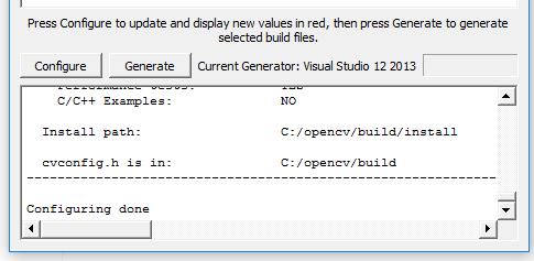
Now, the next thing to do is to configure your build by clicking the Configure button in the CMake window. A pop-up that prompts you to select a compiler will show, choose Visual Studio 12 2013 or the VS version you have installed on your machine. Once chosen, click finish and the configuration process will start. Once its done, the status window should say Configuring done like below:

configure

Once the configuration is complete, you will receive fields marked in red in the above display window. If your result is just a long list of fields, make sure to check the Grouped checkbox so that they are nicely grouped like the image below.
configurecomplete

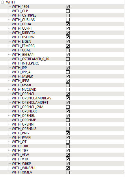
First, the WITH field describes the features you want to include inside your openCV binaries. You can include or exclude a feature by using the checkbox in the list. The defaults should be fine, by this is all up to you. If you want to know what each field does, just hover over them and an explanation will pop up.

with

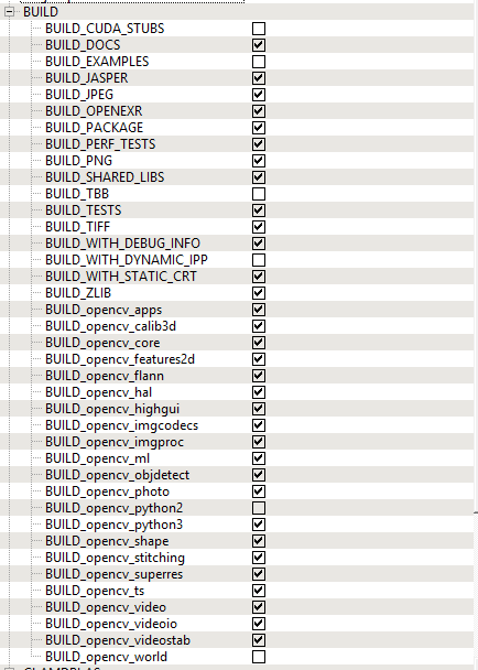
Next, you need to configure the BUILD field. The BUILD field configures the build method used to build the binaries and also the modules that are to be build into the binaries. The fields in ALL CAPS are the build methods and the rest are the modules to be built. You can keep the methods as is. This is also the case for the modules except for one thing. Since we are building for python 3.4+ we do not need to build for python 2+, therefore it is necessary to uncheck the BUILD_opencv_python2 checkbox. If left checked, this will cause an error during the build process if you do not have python 2+ installed in your machine.

buildcmake

Now, that everything is configured, click the Generate button to create the build filesinside the build folder.

Step 5

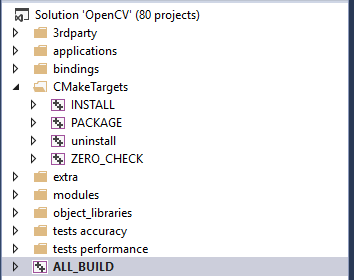
Once the build files have been generated by CMake, the next step is to create the binaries using Visual Studio as the compiler. First, go to the your opencv/build directory, then find and open the openCV solution (opencv.sln). Once the solution is open, you should get a solution explorer that looks something like this

allbuild

Before we build anything, change the build mode to Release instead of Debug. Now,right-click on the Solution ‘OpenCV’ or on ALL_BUILD and select Build. This will start the build process and may take some time.

Once the build is complete, right-click on INSTALL to install openCV-Python on your machine.

Step 6

Once the installation is complete, we need to verify the installation by using python IDLE. Just search for IDLE in the Start Menu and run the program. Type import cv2 in the command line and hit Enter. If no error is found then congratulations, you have just successfully built and installed openCV 3.0 with python 3.4+ bindings on Windows.

idle


Additional Notes:

  • You can also check the openCV version you have installed with python by using the cv2.__version__ command (as shown above).
  • One error I did receive was that the openCV dll could not be found when calling the command import cv2. This can be solved by adding the Release folder created during the build process to your system path (for me, it was C:\opencv\build\bin\Release)
  • In order to code python in Visual Studio, you need to use PTVS (Python Tools for Visual Studio). You can download PTVS from Microsoft’s PTVS page here.

Posted in OpenCV | Tagged: , , | Leave a Comment »

Databases for Multi-camera , Network Camera , E-Surveillace

Posted by Hemprasad Y. Badgujar on February 18, 2016


Multi-view, Multi-Class Dataset: pedestrians, cars and buses

This dataset consists of 23 minutes and 57 seconds of synchronized frames taken at 25fps from 6 different calibrated DV cameras.
One camera was placed about 2m high of the ground, two others where located on a first floor high, and the rest on a second floor to cover an area of 22m x 22m.
The sequence was recorded at the EPFL university campus where there is a road with a bus stop, parking slots for cars and a pedestrian crossing.

Download

Ground truth images
Ground truth annotations

References

The dataset on this page has been used for our multiview object pose estimation algorithm described in the following paper:

G. Roig, X. Boix, H. Ben Shitrit and P. Fua Conditional Random Fields for Multi-Camera Object Detection, ICCV11.

Multi-camera pedestrians video

“EPFL” data set: Multi-camera Pedestrian Videos

people tracking
results, please cite one of the references below.

On this page you can download a few multi-camera sequences that we acquired for developing and testing our people detection and tracking framework. All of the sequences feature several synchronised video streams filming the same area under different angles. All cameras are located about 2 meters from the ground. All pedestrians on the sequences are members of our laboratory, so there is no privacy issue. For the Basketball sequence, we received consent from the team.

Laboratory sequences

These sequences were shot inside our laboratory by 4 cameras. Four (respectively six) people are sequentially entering the room and walking around for 2 1/2 minutes. The frame rate is 25 fps and the videos are encoded using MPEG-4 codec.

[Camera 0] [Camera 1] [Camera 2] [Camera 3]

Calibration file for the 4 people indoor sequence.

[Camera 0] [Camera 1] [Camera 2] [Camera 3]

Calibration file for the 6 people indoor sequence.

Campus sequences

These two sequences called campus were shot outside on our campus with 3 DV cameras. Up to four people are simultaneously walking in front of them. The white line on the screenshots shows the limits of the area that we defined to obtain our tracking results. The frame rate is 25 fps and the videos are encoded using Indeo 5 codec.

[Seq.1, cam. 0] [Seq.1, cam. 1] [Seq.1, cam. 2]
[Seq.2, cam. 0] [Seq.2, cam. 1] [Seq.2, cam. 2]

Calibration file for the two above outdoor scenes.

Terrace sequences

The sequences below, called terrace, were shot outside our building on a terrace. Up to 7 people evolve in front of 4 DV cameras, for around 3 1/2 minutes. The frame rate is 25 fps and the videos are encoded using Indeo 5 codec.

[Seq.1, cam. 0] [Seq.1, cam. 1] [Seq.1, cam. 2] [Seq.1, cam. 3]
[Seq.2, cam. 0] [Seq.2, cam. 1] [Seq.2, cam. 2] [Seq.1, cam. 3]

Calibration file for the terrace scene.

Passageway sequence

This sequence dubbed passageway was filmed in an underground passageway to a train station. It was acquired with 4 DV cameras at 25 fps, and is encoded with Indeo 5. It is a rather difficult sequence due to the poor lighting.

[Seq.1, cam. 0] [Seq.1, cam. 1] [Seq.1, cam. 2] [Seq.1, cam. 3]

Calibration file for the passageway scene.

Basketball sequence

This sequence was filmed at a training session of a local basketball team. It was acquired with 4 DV cameras at 25 fps, and is encoded with Indeo 5.

[Seq.1, cam. 0] [Seq.1, cam. 1] [Seq.1, cam. 2] [Seq.1, cam. 3]

Calibration file for the basketball scene.

Camera calibration

POM only needs a simple calibration consisting of two homographies per camera view, which project the ground plane in top view to the ground plane in camera views and to the head plane in camera views (a plane parallel to the ground plane but located 1.75 m higher). Therefore, the calibration files given above consist of 2 homographies per camera. In degenerate cases where the camera is located inside the head plane, this one will project to a horizontal line in the camera image. When this happens, we do not provide a homography for the head plane, but instead we give the height of the line in which the head plane will project. This is expressed in percentage of the image height, starting from the top.

The homographies given in the calibration files project points in the camera views to their corresponding location on the top view of the ground plane, that is

H * X_image = X_topview .

We have also computed the camera calibration using the Tsai calibration toolkit for some of our sequences. We also make them available for download. They consist of an XML file per camera view, containing the standard Tsai calibration parameters. Note that the image size used for calibration might differ from the size of the video sequences. In this case, the image coordinates obtained with the calibration should be normalized to the size of the video.

Ground truth

We have created a ground truth data for some of the video sequences presented above, by locating and identifying the people in some frames at a regular interval.

To use these ground truth files, you must rely on the same calibration with the exact same parameters that we used when generating the data. We call top view the rectangular area of the ground plane in which we perform tracking.

This area is of dimensions tv_width x tv_height and has top left coordinate (tv_origin_x, tv_origin_y). Besides, we call grid our discretization of the top view area into grid_width x grid_height cells. An example is illustrated by the figure below, in which the grid has dimensions 5 x 4.

The people’s position in the ground truth are expressed in discrete grid coordinates. In order to be projected into the images with homographies or the Tsai calibration, these grid coordinates need to be translated into top view coordinates. We provide below a simple C function that performs this translation. This function takes the following parameters:

  • pos : the person position coming from the ground truth file
  • grid_width, grid_height : the grid dimension
  • tv_origin_x, tv_origin_y : the top left corner of the top view
  • tv_width, tv_height : the top view dimension
  • tv_x, tv_y : the top view coordinates, i.e. the output of the function
  void grid_to_tv(int pos, int grid_width, int grid_height,                  float tv_origin_x, float tv_origin_y, float tv_width,                  float tv_height, float &tv_x, float &tv_y) {     tv_x = ( (pos % grid_width) + 0.5 ) * (tv_width / grid_width) + tv_origin_x;    tv_y = ( (pos / grid_width) + 0.5 ) * (tv_height / grid_height) + tv_origin_y;  }

The table below summarizes the aforementionned parameters for the ground truth files we provide. Note that the ground truth for the terrace sequence has been generated with the Tsai calibration provided in the table. You will need to use this one to get a proper bounding box alignment.

Ground Truth Grid dimensions Top view origin Top view dimensions Calibration
6-people laboratory 56 x 56 (0 , 0) 358 x 360 file
terrace, seq. 1 30 x 44 (-500 , -1,500) 7,500 x 11,000 file (Tsai)
passageway, seq. 1 40 x 99 (0 , 38.48) 155 x 381 file

The format of the ground truth file is the following:

 1 <number of frames>  <number of people>  <grid width>  <grid height>  <step size>  <first frame>  <last frame> <pos> <pos> <pos> ... <pos> <pos> <pos> ... . . .

where <number of frames> is the total number of frames, <number of people> is the number of people for which we have produced a ground truth, <grid width> and <grid height>are the ground plane grid dimensions, <step size> is the frame interval between two ground truth labels (i.e. if set to 25, then there is a label once every 25 frames), and <first frame> and <last frame> are the first and last frames for which a label has been entered.

After the header, every line represents the positions of people at a given frame. <pos> is the position of a person in the grid. It is normally a integer >= 0, but can be -1 if undefined (i.e. no label has been produced for this frame) or -2 if the person is currently out of the grid.

References

Multiple Object Tracking using K-Shortest Paths Optimization

Jérôme Berclaz, François Fleuret, Engin Türetken, Pascal Fua
IEEE Transactions on Pattern Analysis and Machine Intelligence
2011
pdf | show bibtex

Multi-Camera People Tracking with a Probabilistic Occupancy Map

François Fleuret, Jérôme Berclaz, Richard Lengagne, Pascal Fua
IEEE Transactions on Pattern Analysis and Machine Intelligence
pdf | show bibtex

MuHAVi: Multicamera Human Action Video Data

including selected action sequences with

MAS: Manually Annotated Silhouette Data

for the evaluation of human action recognition methods

Figure 1. The top view of the configuration of 8 cameras used to capture the actions in the blue action zone (which is marked with white tapes on the scene floor).

camera symbol

camera name

V1 Camera_1
V2 Camera_2
V3 Camera_3
V4 Camera_4
V5 Camera_5
V6 Camera_6
V7 Camera_7
V8 Camera_8

Table 1. Camera view names appearing in the MuHAVi data folders and the corresponding symbols used in Fig. 1.


On the table below, you can click on the links to download the data (JPG images) for the corresponding action

Important: We noted that some earlier versions of that earlier versions of MS Internet Explorer could not download files over 2GB size, so we recomment to use alternative browsers such as Firefox or Chrome.

Each tar file contains 7 folders corresponding to 7 actors (Person1 to Person7) each of which contains 8 folders corresponding to 8 cameras (Camera_1 to Camera_8). Image frames corresponding to every combination of action/actor/camera are named with image frame numbers starting from 00000001.jpg for simplicity. The video frame rate is 25 frames per second and the resolution of image frames (except for Camera_8) is 720 x 576 Pixels (columns x rows). The image resolution is 704 x 576 for Camera_8.

action class

action name

size
C1 WalkTurnBack 2.6GB
C2 RunStop 2.5GB
C3 Punch 3.0GB
C4 Kick 3.4GB
C5 ShotGunCollapse 4.3GB
C6 PullHeavyObject 4.5GB
C7 PickupThrowObject 3.0GB
C8 WalkFall 3.9GB
C9 LookInCar 4.6GB
C10 CrawlOnKnees 3.4GB
C11 WaveArms 2.2GB
C12 DrawGraffiti 2.7GB
C13 JumpOverFence 4.4GB
C14 DrunkWalk 4.0GB
C15 ClimbLadder 2.1GB
C16 SmashObject 3.3GB
C17 JumpOverGap 2.6GB

MIT Trajectory Data Set – Multiple Camera Views

Download

MIT trajectory data set is for the research of activity analysis in multiple single camera view using the trajectories of objects as features. Object tracking is based on background subtraction using a Adaptive Gaussian Mixture model. There are totally four camera views. Trajectories in different camera views have been synchronized. The data can be downloaded from the following link,

MIT trajectory data set

Background image

Reference

Please cite as:

X. Wang, K. Tieu and E. Grimson, Correspondence‐Free Activity Analysis and Scene Modeling in Multiple Camera Views, IEEE Transactions on Pattern Analysis and Machine Intelligence(PAMI), Vol. 32, pp. 56-71, 2010..

Details

MIT traffic data set is for research on activity analysis and crowded scenes. It includes a traffic video sequence of 90 minutes long. It is recorded by a stationary camera. The size of the scene is 720 by 480. It is divided into 20 clips and can be downloaded from the following links.

Ground Truth

In order to evaluate the performance of human detection on this data set, ground truth of pedestrians of some sampled frames are manually labeled. It can be downloaded below. A readme file provides the instructions of how to use it.
Ground truth of pedestrians

References

  1. Unsupervised Activity Perception in Crowded and Complicated scenes Using Hierarchical Bayesian Models
    X. Wang, X. Ma and E. Grimson
    IEEE Transactions on Pattern Analysis and Machine Intelligence (PAMI), Vol. 31, pp. 539-555, 2009
  2. Automatic Adaptation of a Generic Pedestrian Detector to a Specific Traffic Scene
    M. Wang and X. Wang
    IEEE Computer Society Conference on Computer Vision and Pattern Recognition (CVPR), 2011

Description

This dataset is presented in our CVPR 2015 paper,
Linjie Yang, Ping Luo, Chen Change Loy, Xiaoou Tang. A Large-Scale Car Dataset for Fine-Grained Categorization and Verification, In Computer Vision and Pattern Recognition (CVPR), 2015. PDF

The Comprehensive Cars (CompCars) dataset contains data from two scenarios, including images from web-nature and surveillance-nature. The web-nature data contains 163 car makes with 1,716 car models. There are a total of 136,726 images capturing the entire cars and 27,618 images capturing the car parts. The full car images are labeled with bounding boxes and viewpoints. Each car model is labeled with five attributes, including maximum speed, displacement, number of doors, number of seats, and type of car. The surveillance-nature data contains 50,000 car images captured in the front view. Please refer to our paper for the details.

The dataset is well prepared for the following computer vision tasks:

  • Fine-grained classification
  • Attribute prediction
  • Car model verification

The train/test subsets of these tasks introduced in our paper are included in the dataset. Researchers are also welcome to utilize it for any other tasks such as image ranking, multi-task learning, and 3D reconstruction.

Note

  1. You need to complete the release agreement form to download the dataset. Please see below.
  2. The CompCars database is available for non-commercial research purposes only.
  3. All images of the CompCars database are obtained from the Internet which are not property of MMLAB, The Chinese University of Hong Kong. The MMLAB is not responsible for the content nor the meaning of these images.
  4. You agree not to reproduce, duplicate, copy, sell, trade, resell or exploit for any commercial purposes, any portion of the images and any portion of derived data.
  5. You agree not to further copy, publish or distribute any portion of the CompCars database. Except, for internal use at a single site within the same organization it is allowed to make copies of the database.
  6. The MMLAB reserves the right to terminate your access to the database at any time.
  7. All submitted papers or any publicly available text using the CompCars database must cite the following paper:
    Linjie Yang, Ping Luo, Chen Change Loy, Xiaoou Tang. A Large-Scale Car Dataset for Fine-Grained Categorization and Verification, In Computer Vision and Pattern Recognition (CVPR), 2015.

Download instructions

Download the CompCars dataset Release Agreement, read it carefully, and complete it appropriately. Note that the agreement should be signed by a full-time staff member (that is, student is not acceptable). Then, please scan the signed agreement and send it to Mr. Linjie Yang (yl012(at)ie.cuhk.edu.hk) and cc to Chen Change Loy (ccloy(at)ie.cuhk.edu.hk). We will verify your request and contact you on how to download the database.

Stanford Cars Dataset

Overview

       The Cars dataset contains 16,185 images of 196 classes of cars. The data is split into 8,144 training images and 8,041 testing images, where each class has been split roughly in a 50-50 split. Classes are typically at the level of Make, Model, Year, e.g. 2012 Tesla Model S or 2012 BMW M3 coupe.

Download

       Training images can be downloaded here.
Testing images can be downloaded here.
A devkit, including class labels for training images and bounding boxes for all images, can be downloaded here.
If you’re interested in the BMW-10 dataset, you can get that here.

Update: For ease of development, a tar of all images is available here and all bounding boxes and labels for both training and test are available here. If you were using the evaluation server before (which is still running), you can use test annotations here to evaluate yourself without using the server.

Evaluation

       An evaluation server has been set up here. Instructions for the submission format are included in the devkit. This dataset was featured as part of FGComp 2013, and competition results are directly comparable to results obtained from evaluating on images here.

Citation

       If you use this dataset, please cite the following paper:

3D Object Representations for Fine-Grained Categorization
Jonathan Krause, Michael Stark, Jia Deng, Li Fei-Fei
4th IEEE Workshop on 3D Representation and Recognition, at ICCV 2013 (3dRR-13). Sydney, Australia. Dec. 8, 2013.
[pdf]   [BibTex]   [slides]

Note that the dataset, as released, has 196 categories, one less than in the paper, as it has been cleaned up slightly since publication. Numbers should be more or less comparable, though.

The HDA dataset is a multi-camera high-resolution image sequence dataset for research on high-definition surveillance. 18 cameras (including VGA, HD and Full HD resolution) were recorded simultaneously during 30 minutes in a typical indoor office scenario at a busy hour (lunch time) involving more than 80 persons. In the current release (v1.1), 13 cameras have been fully labeled.


The venue spans three floors of the Institute for Systems and Robotics (ISR-Lisbon) facilities. The following pictures show the placement of the cameras. The 18 recorded cameras are identified with a small red circle. The 13 cameras with a coloured view field have been fully labeled in the current release (v1.1).


Each frame is labeled with the bounding boxes tightly adjusted to the visible body of the persons, the unique identification of each person, and flag bits indicating occlusion and crowd:

  • The bounding box is drawn so that it completely and tightly encloses the person.
  • If the person is occluded by something (except image boundaries), the bounding box is drawn by estimating the whole body extent.
  • People partially outside the image boundaries have their BB’s cropped to image limits. Partially occluded people and people partially outside the image boundaries are marked as ‘occluded’.
  • A unique ID is associated to each person, e.g., ‘person01’. In case of identity doubt, the special ID ‘personUnk’ is used.
  • Groups of people that are impossible to label individually are labelled collectively as ‘crowd’. People in front of a ’crowd’ area are labeled normally.

The following figures show examples of labeled frames: (a) an unoccluded person; (b) two occluded people; (c) a crowd with three people in front.


Data formats:

For each camera we provide the .jpg frames sequentially numbered and a .txt file containing the annotations according to the “video bounding box” (vbb) format defined in the Caltech Pedestrian Detection Database. Also on this site there are tools to visualise the annotations overlapped on the image frames.


Some statistics:

Labeled Sequences: 13

Number of Frames: 75207

Number of Bounding Boxes: 64028

Number of Persons: 85


Repository of Results:

We maintain a public repository of re-identification results in this dataset. Send us your CMC curve to be uploaded  (alex at isr ist utl pt).
Click here to see the full list and detailed experiments.

MANUAL_c_l_e_a_n cam60

Posted in Computer Network & Security, Computer Research, Computer Vision, Image Processing, Multimedia | Leave a Comment »

How to use Twitter as a scientist

Posted by Hemprasad Y. Badgujar on February 5, 2016


fwis-loreal-10-women-scientists-you-should-follow-on-twitter-264.jpg

if you are a scientist, with “joining Twitter” and then “doing stuff with Twitter” on your To Do list, you might feel a little intimidated by the long list of possible people to follow. Moreover, following @CNN and @BarackObama might be the first thing you do, and might be suggested to you, but these are not your main sources of scientific joy and information.

So let’s take this step by step. Let’s go from setting up a profile, following people to building an academic network on Twitter. I don’t want this to become like a tutorial (there’s plenty of videos on YouTube to take you through any step you might have difficulties with), but I want to give you some tips and tricks at every step along the process.

1. Crafting a bio
One of the first things you need to do when you sign up on Twitter, is to put a bio. I recommend that you make your Twitter profile publicly accessible instead of private. If you join Twitter to enter the realm of scientists on Twitter, you’d prefer them to be able to find you and follow you. Make sure your bio mentions your field and institution(s). You can add a warning that Retweets are not Endorsements, but, really, most of the Twitterverse is aware of that.

Keep in mind as well that Twitter is a lighter type of platform. There’s no need for you to cite your recent publications in your bio. I like to add a bit of lightness to my bio by adding “Blogs. Pets cats. Drinks tea.” I’m assuming that also sets up people for the fact that besides the concrete and the science, I could blurt out the odd complaint, random observation or retweet cute cat pictures if I feel like. Does that make me unprofessional? I’m on the border of Gen Y and I don’t think so…

2. Choosing a profile picture
Your standard profile picture is an egg. Whenever I get followed by an egg, I don’t even take the effort to read the profile description of this person, because the sole fact that he/she didn’t even finish his/her profile, makes me doubt this person has any real interest in interacting on Twitter.

Since Twitter profile pictures show up very small, I recommend you use a headshot. If you put a full body picture of yourself presenting your work somewhere, you’ll be reduced to the size of a stickman in people’s timelines. Use a clear, recognizable headshot, so that the odd fellow researcher might be able to recognize you at a conference.

3. Following people

So now that we have the basics covered, let’s start to move forward into the actual use of Twitter. Your first recommended people to follow will typically be @CNN and @BarackObama. While I like using Twitter as a source for the news, I’m going to assume you came here in the first place for the scientific community. How do you start following people?

Here are a few types of accounts that you can/should start following:
– the accounts of your university and department. These accounts will also retweet tweets from fellow academics at your institute.
– the accounts of universities and research groups worldwide you are interested in.
– the accounts of academic publishers
– the accounts of news websites and blogs related with higher education, such as @insidehighered
– make a search for your field and see what and who shows up
– organizations in your field
– Twitter lists about your field or with people from your institution

Keep in mind that, just like growing followers, growing a list of interesting people to follow is something that happens over time. You might see a retweet of somebody, check out his/her profile and then decide to follow this tweep. If you start aggressively following a lot of people in a short amount of time, Twitter will ban you from following more people anyway.

4. Creating content
Now you can start creating content. You can tweet about your recent publications, retweet information from the accounts you follow and more. If you have a blog, Twitter is an excellent place to share your recent blog posts. You can also tweet series of posts (indicated by (1/3), (2/3) and (3/3) if you distribute it over 3 posts, for example) of the contents that you want to share is too long to squeeze into 150 characters.

Some ideas on what to share with the world:
– tweet about the topic you will discuss in class
– tweet about the conference you are planning to attend
– share your progress in writing
– talk about a recent publication
– join the discussion about higher education policies (I know you have an opinion – we all do)

5. Getting the discussion started
If you see a topic of your interest, you don’t need to wait for anyone to invite you to take part in the discussion – you can imply barge right into it. You wouldn’t do it in real life, but on Twitter, nobody knows you are reading along. So comment to what fellow researchers are sharing, ask for ideas and opinions and interact.

You can also tag people in a post by adding their @name when you share an article and ask what they think. In this way, you can as well get involved in the academic online discussion.

6. Using hashtags
Hashtags, those #selfie #dinner #random stuff that you see showing up around most social media platforms come from Twitter, where feeds and discussions center around certain hashtags. In the academic world, I recommend you to check out #phdchat, #ecrchat (for early career researchers), #scholarsunday (on Sundays, to learn who to follow), #acwri (for academic writing) and #acwrimo (in November, the month in which academics worldwide pledge to get their manuscript out and post their daily word counts).

Some hashtags have a weekly fixed hour to chat. Other hashtags are continuous streams of information. Figure out what the important hashtags are in your field and in academia in general, listen in and contribute.

7. Saving conversations with Storify

If you had a particularly interesting conversation on Twitter that you would like to save for future reference, you can use Storify. Storify is a website on which you can save stories, by adding social media content. You can, for example, add tweets and replies to tweets in a logical order, to save a discussion you had. Once you finished compiling your story, you can share it again through social media. Stories also remain saved and accessible for the future in Storify.

8. Curating content
Retweeting, sharing articles, hosting people to write on your blog, … all these activities are related to curating content and broadcasting it to your audience. I enjoy interviewing fellow academics that I meet through Twitter. I post the interview then on my blog, and share that link on Twitter (going full circle). From a number of newsletters that I read, I also share articles and interesting documents. Find out what type of content you and your followers find relevant, and start distributing interesting information.

Posted in Computing Technology, Mixed, My Research Related | Tagged: , , , , | Leave a Comment »

HOW TO PASS COMMAND-LINE ARGUMENTS IN ECLIPSE IDE?

Posted by Hemprasad Y. Badgujar on November 30, 2015


New Java Project

  • Create a new Java Project and name it as “CommandLineArguments

Right click on Package Explorer -> New -> Project -> Select Java Project

New package

  • Create a new Package and name it as “commandline

Right click on src -> New -> Package

New Class

  • Create a new Java Class and name it as “AdditionOfTwoNumbers” in the package “commandline“. Make sure you select main method option.

Right click on commandline package -> New -> Class

Paste this code in the main method.

01
02
03
04
05
06
07
08
09
10
11
package commandline;
public class AdditionOfTwoNumbers {
    public static void main(String[] args) {
        int a, b;
        a = Integer.parseInt(args[0]);
        b = Integer.parseInt(args[1]);
        
        int sum = a + b;
        System.out.println("The Sum is: " + sum);
    }
}

Save the program.

  • Press [Ctrl + s] to save your program

Run Configurations

Go to Run menu and select Run Configurations. Run Configurations dialogue box opens.

Run your program

  • Select your Java class from the left side column. If you do not find your class, then click on the “New launch Configuration” button, found above the class list.
  • In the right side menu select “Arguments” tab
  • In the “Program Arguments” text area type the input numbers separated by spaces or newline.
  • Click Run button.

Output

  • You will see the output in the console.

The Sum is: 32

Posted in Mixed | Leave a Comment »

CUDA Unified Memory

Posted by Hemprasad Y. Badgujar on October 6, 2015


CUDA Unified Memory

CUDA is the language of Nvidia GPU’s.  To extract maximum performance from GPU’s, you’ll want to develop applications in CUDA.

CUDA Toolkit is the primary IDE (integrated development environment) for developing CUDA-enabled applications.  The main roles of the Toolkit IDE are to simplify the software development process, maximize software developer productivity, and provide features that enhance GPU performance.  The Toolkit has been steadily evolving in tandem with GPU hardware and currently sits at Version 6.5.

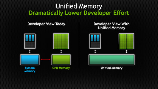
One of the most important features of CUDA 6.5 is Unified Memory (UM).  (UM was actually first introduced in CUDA v.6.0).  CPU host memory and GPU device memory are physically separate entities, connected by a relatively slow PCIe bus.  Prior to v.6.0, data elements shared in both CPU and GPU memory required two copies – one copy in CPU memory and one copy in GPU memory.  Developers had to allocate memory on the CPU, allocate memory on the GPU, and then copy data from CPU to GPU and from GPU to CPU.  This dual data management scheme added complexity to programs, opportunities for the introduction of software bugs, and an excessive focus of time and energy on data management tasks.

UM corrects this.  UM creates a memory pool that is shared between CPU and GPU, with a single memory address space and single pointers accessible to both host and device code.  The CUDA driver and runtime libraries automatically handle data transfers between host and device memory, thus relieving developers from the burden of explicitly managing those data transfers.  UM improves performance by automatically providing data locality on the CPU or GPU, wherever it might be required by the application algorithm.  UM also guarantees global coherency of data on host and device, thus reducing the introduction of software bugs.

Let’s explore some sample code that illustrates these concepts.  We won’t concern ourselves with the function of this algorithm; instead, we’ll just focus on the syntax. (Credit to Nvidia for this C/CUDA template example).

Without Unified Memory

Without Unified Memory

1
2
3
4
5
6
7
8
9
10
11
12
13
14
15
16
17
18
19
20
21
22
23
24
25
26
27
28
29
30
31
32
33
34
35
36
37
38
39
40
41
42
43
44
45
46
47
48
49
50
51
52
53
54
55
56
57
58
59
60
61
62
63
64
65
#include <string.h>
#include <stdio.h>
struct DataElement
{
  char *name;
  int value;
};
__global__
void Kernel(DataElement *elem) {
  printf("On device: name=%s, value=%d\n", elem->name, elem->value;
  elem->name[0] = 'd';
  elem->value++;
}
void launch(DataElement *elem) {
  DataElement *d_elem;
  char *d_name;
  int namelen = strlen(elem->name) + 1;
  // Allocate memory on GPU
  cudaMalloc(&d_elem, sizeofDataElement());
  cudaMalloc(&d_name, namelen);
  // Copy data from CPU to GPU
  cudaMemcpy(d_elem, elem, sizeof(DataElement),
     cudaMemcpyHostToDevice);
  cudaMemcpy(d_name, elem->name, namelen, cudaMemcpyHostToDevice);
  cudaMemcpy(&(d_elem->name), &d_name, sizeof(char*),
     cudaMemcpyHostToDevice);
  // Launch kernel
  Kernel<<< 1, 1 >>>(d_elem);
  // Copy data from GPU to CPU
  cudaMemcpy(&(elem->value), &(d_elem->value), sizeof(int),
     cudaMemcpyDeviceToHost);
  cudaMemcpy(elem->name, d_name, namelen, cudaMemcpyDeviceToHost);
  cudaFree(d_name);
  cudaFree(d_elem);
}
int main(void)
{
  DataElement *e;
  // Allocate memory on CPU
  e = (DataElement*)malloc(sizeof(DataElement));
  e->value = 10;
  // Allocate memory on CPU
  e->name = (char*)malloc(sizeof(char) * (strlen("hello") + 1));
  strcpy(e->name, "hello");
  launch(e);
  printf("On host: name=%s, value=%d\n", e->name, e->value);
  free(e->name);
  free(e);
  cudaDeviceReset();
}

Note these key points:

  • L51,55: Allocate memory on CPU
  • L24,25: Allocate memory on GPU
  • L28-32: Copy data from CPU to GPU
  • L35: Run kernel
  • L38-40: Copy data from GPU to CPU

With Unified Memory 

1
2
3
4
5
6
7
8
9
10
11
12
13
14
15
16
17
18
19
20
21
22
23
24
25
26
27
28
29
30
31
32
33
34
35
36
37
38
39
40
41
42
43
44
#include <string.h>
#include <stdio.h>
struct DataElement
{
  char *name;
  int value;
};
__global__
void Kernel(DataElement *elem) {
  printf("On device: name=%s, value=%d\n", elem->name, elem->value;
  elem->name[0] = 'd';
  elem->value++;
}
void launch(DataElement *elem) {
  // Launch kernel
  Kernel<<< 1, 1 >>>(elem);
  cudaDeviceSynchronize();
}
int main(void)
{
  DataElement *e;
  // Allocate unified memory on CPU and GPU
  cudaMallocManaged((void**)&e, sizeof(DataElement));
  e->value = 10;
  // Allocate unified memory on CPU and GPU
  cudaMallocManaged((void**)&(e->name), sizeof(char) *
     (strlen("hello") + 1) );
  strcpy(e->name, "hello");
  launch(e);
  printf("On host: name=%s, value=%d\n", e->name, e->value);
  cudaFree(e->name);
  cudaFree(e);
  cudaDeviceReset();
}
 

Note these key points:

  • L28, 32, 33: Allocate unified memory on CPU and GPU
  • L19: Run kernel

With UM, memory is allocated on the CPU and GPU in a single address space and managed with a single pointer.  Note how the “malloc’s” and “cudaMalloc’s” are condensed into single calls to cudaMallocManaged().  Furthermore, explicit cudaMemcpy() data transfers between CPU and GPU are eliminated, as the CUDA runtime handles these transfers automatically in the background. Collectively these actions simplify code development, code maintenance, and data management.

As software project managers, we like UM for the productivity enhancements it provides for our software development teams.  It improves software quality, reduces coding time, effort and cost, and enhances overall performance. As software engineers, we like UM because of reduced coding effort and the fact that we can focus time and effort on writing CUDA kernel code, where all the parallel performance comes from, instead of spending time on memory management tasks.  Unified Memory is major step forward in GPU programming.

Posted in CUDA, CUDA TUTORIALS, GPU (CUDA), PARALLEL | Leave a Comment »

CUDA Random Numbers

Posted by Hemprasad Y. Badgujar on October 3, 2015


CUDA Random Example

In order to use cuRAND, we need to add two include files into our program:

#include &lt;curand.h&gt;
#include &lt;curand_kernel.h&gt;

cuRAND uses a curandState_t type to keep track of the state of the random sequence. The normal C rand function also has a state, but it is global, and hidden from the programmer. This makes rand not thread-safe, but easier to use.

A curandState_t object must be initialized with a call to curand_init which has the following parameters:

  • seed: The seed determines the beginning point of the sequence of random numbers.
  • sequence: The sequence number is another seed-like value. It is used so that, if all cores have the same seed, but different sequence numbers, then they will get different random values.
  • offset: The amount we skip ahead in the random sequence. This can be zero.
  • state: A pointer to the curandState_t object to initialize.

Once we have an initialized curandState_t object, we can get random numbers with the curand function which takes a pointer to a curandState_t object and returns to us a random unsigned integer.

The following program uses these functions to generate random numbers:

#include <unistd.h>
#include <stdio.h>

/* we need these includes for CUDA's random number stuff */
#include <curand.h>
#include 

#define MAX 100

/* this GPU kernel function calculates a random number and stores it in the parameter */
__global__ void random(int* result) {
  /* CUDA's random number library uses curandState_t to keep track of the seed value
     we will store a random state for every thread  */
  curandState_t state;

  /* we have to initialize the state */
  curand_init(0, /* the seed controls the sequence of random values that are produced */
              0, /* the sequence number is only important with multiple cores */
              0, /* the offset is how much extra we advance in the sequence for each call, can be 0 */
              &state);

  /* curand works like rand - except that it takes a state as a parameter */
  *result = curand(&state) % MAX;
}

int main( ) {
  /* allocate an int on the GPU */
  int* gpu_x;
  cudaMalloc((void**) &gpu_x, sizeof(int));

  /* invoke the GPU to initialize all of the random states */
  random<<<1, 1>>>(gpu_x);

  /* copy the random number back */
  int x;
  cudaMemcpy(&x, gpu_x, sizeof(int), cudaMemcpyDeviceToHost);

  printf("Random number = %d.\n", x);

  /* free the memory we allocated */
  cudaFree(gpu_x);

  return 0;
}

When run, this program produces the exact same random number each time. This is because the seed passed in was 0. In order to get a different random number each time, we can pass in the current time as the seed.


#include <unistd.h>
#include <stdio.h>

/* we need these includes for CUDA's random number stuff */

#include 
#include 

#define MAX 100

/* this GPU kernel function calculates a random number and stores it in the parameter */
__global__ void random(unsigned int seed, int* result) {
  /* CUDA's random number library uses curandState_t to keep track of the seed value
     we will store a random state for every thread  */
  curandState_t state;

  /* we have to initialize the state */
  curand_init(seed, /* the seed controls the sequence of random values that are produced */
              0, /* the sequence number is only important with multiple cores */
              0, /* the offset is how much extra we advance in the sequence for each call, can be 0 */
              &state);

  /* curand works like rand - except that it takes a state as a parameter */
  *result = curand(&state) % MAX;
}

int main( ) {
  /* allocate an int on the GPU */
  int* gpu_x;
  cudaMalloc((void**) &gpu_x, sizeof(int));

  /* invoke the GPU to initialize all of the random states */
  random<<<1, 1>>>(time(NULL), gpu_x);

  /* copy the random number back */
  int x;
  cudaMemcpy(&x, gpu_x, sizeof(int), cudaMemcpyDeviceToHost);

  printf("Random number = %d.\n", x);

  /* free the memory we allocated */
  cudaFree(gpu_x);

  return 0;
}

Using Random Numbers Across Cores

If we want to get random numbers in multiple GPU cores, then we would need each core to have its own curandState_t.

If we want each run of the program to produce different sequences of random numbers, then we would need to set the seed to the current time.

However, now we would likely have each core get the same sequence of numbers. This is probably undesirable. To avoid it, we set the sequence parameter to the thread’s ID.

This way, each thread will have a different stream of random numbers, which will also be different each time the program is run.

The following program illustrates this by creating N curandState_t objects, then launching a GPU kernel to get N random numbers from them, in parallel.

#include <unistd.h>
#include <stdio.h>

/* we need these includes for CUDA's random number stuff */
#include 
#include 

#define N 25

#define MAX 100

/* this GPU kernel function is used to initialize the random states */
__global__ void init(unsigned int seed, curandState_t* states) {

  /* we have to initialize the state */
  curand_init(seed, /* the seed can be the same for each core, here we pass the time in from the CPU */
              blockIdx.x, /* the sequence number should be different for each core (unless you want all
                             cores to get the same sequence of numbers for some reason - use thread id! */
              0, /* the offset is how much extra we advance in the sequence for each call, can be 0 */
              &states[blockIdx.x]);
}

/* this GPU kernel takes an array of states, and an array of ints, and puts a random int into each */
__global__ void randoms(curandState_t* states, unsigned int* numbers) {
  /* curand works like rand - except that it takes a state as a parameter */
  numbers[blockIdx.x] = curand(&states[blockIdx.x]) % 100;
}

int main( ) {
  /* CUDA's random number library uses curandState_t to keep track of the seed value
     we will store a random state for every thread  */
  curandState_t* states;

  /* allocate space on the GPU for the random states */
  cudaMalloc((void**) &states, N * sizeof(curandState_t));

  /* invoke the GPU to initialize all of the random states */
  init<<<n, 1="">>>(time(0), states);

  /* allocate an array of unsigned ints on the CPU and GPU */
  unsigned int cpu_nums[N];
  unsigned int* gpu_nums;
  cudaMalloc((void**) &gpu_nums, N * sizeof(unsigned int));

  /* invoke the kernel to get some random numbers */
  randoms<<<n, 1="">>>(states, gpu_nums);

  /* copy the random numbers back */
  cudaMemcpy(cpu_nums, gpu_nums, N * sizeof(unsigned int), cudaMemcpyDeviceToHost);

  /* print them out */
  for (int i = 0; i < N; i++) {
    printf("%u\n", cpu_nums[i]);
  }

  /* free the memory we allocated for the states and numbers */
  cudaFree(states);
  cudaFree(gpu_nums);

  return 0;
}

This program is also the first to use multiple GPU kernel functions.


Random Distributions

In addition to the curand function which, together with modular arithmetic, can return to us random integers from any range we wish, cuRAND provides functions to get floating point numbers from different distributions:

__device__ float curand_uniform (curandState_t *state)

__device__ float curand_normal (curandState_t *state)

curand_uniform returns a random number between 0.0 and 1.0 following a uniform distribution. This means that all floating point numbers in that range are equally likely to be produced.

curand_normal also returns a random number between 0.0 and 1.0, but it follows a normal distribution, meaning that the number 0.5 is more likely to be produced than numbers near 0.0 or 1.0. Normal distributions would be important for modelling many natural phenomenon accurately.

Posted in CUDA TUTORIALS, GPU (CUDA), PARALLEL | Tagged: | Leave a Comment »

Bilateral Filtering

Posted by Hemprasad Y. Badgujar on September 14, 2015


Popular Filters

When smoothing or blurring images (the most popular goal of smoothing is to reduce noise), we can use diverse linear filters, because linear filters are easy to achieve, and are kind of fast, the most used ones are Homogeneous filter, Gaussian filter, Median filter, et al.

When performing a linear filter, we do nothing but output pixel’s value g(i,j)  which is determined as a weighted sum of input pixel values f(i+k, j+l):

g(i, j)=SUM[f(i+k, j+l) h(k, l)];

in which, h(k, l)) is called the kernel, which is nothing more than the coefficients of the filter.

Homogeneous filter is the most simple filter, each output pixel is the mean of its kernel neighbors ( all of them contribute with equal weights), and its kernel K looks like:

1

 Gaussian filter is nothing but using different-weight-kernel, in both x and y direction, pixels located in the middle would have bigger weight, and the weights decrease with distance from the neighborhood center, so pixels located on sides have smaller weight, its kernel K is something like (when kernel is 5*5):

gkernel

Median filter is something that replace each pixel’s value with the median of its neighboring pixels. This method is great when dealing with “salt and pepper noise“.

Bilateral Filter

By using all the three above filters to smooth image, we not only dissolve noise, but also smooth edges, which make edges less sharper, even disappear. To solve this problem, we can use a filter called bilateral filter, which is an advanced version of Gaussian filter, it introduces another weight that represents how two pixels can be close (or similar) to one another in value, and by considering both weights in image,  Bilateral filter can keep edges sharp while blurring image.

Let me show you the process by using this image which have sharp edge.

21


Say we are smoothing this image (we can see noise in the image), and now we are dealing with the pixel at middle of the blue rect.

22   23

Left-above picture is a Gaussian kernel, and right-above picture is Bilateral filter kernel, which considered both weight.

We can also see the difference between Gaussian filter and Bilateral filter by these pictures:

Say we have an original image with noise like this

32


By using Gaussian filter, the image is smoother than before, but we can see the edge is no longer sharp, a slope appeared between white and black pixels.

33


However, by using Bilateral filter, the image is smoother, the edge is sharp, as well.

31

OpenCV code

It is super easy to make these kind of filters in OpenCV:

1 //Homogeneous blur:
2 blur(image, dstHomo, Size(kernel_length, kernel_length), Point(-1,-1));
3 //Gaussian blur:
4 GaussianBlur(image, dstGaus, Size(kernel_length, kernel_length), 0, 0);
5 //Median blur:
6 medianBlur(image, dstMed, kernel_length);
7 //Bilateral blur:
8 bilateralFilter(image, dstBila, kernel_length, kernel_length*2, kernel_length/2);

and for each function, you can find more details in OpenCV Documentation

Test Images

Glad to use my favorite Van Gogh image :

vangogh


From left to right: Homogeneous blur, Gaussian blur, Median blur, Bilateral blur.

(click iamge to view full size version :p )

kernel length = 3:

homo3 Gaussian3 Median3 Bilateral3

kernel length = 9:

homo9 Gaussian9 Median9 Bilateral9
kernel length = 15:

homo15 Gaussian15 Median15 Bilateral15

kernel length = 23:

homo23 Gaussian23 Median23 Bilateral23
kernel length = 31:

homo31 Gaussian31 Median31 Bilateral31
kernel length = 49:

homo49 Gaussian49 Median49 Bilateral49
kernel length = 99:

homo99 Gaussian99 Median99 Bilateral99

Trackback URL.

Posted in C, Image / Video Filters, Image Processing, OpenCV, OpenCV, OpenCV Tutorial | Leave a Comment »

 
Extracts from a Personal Diary

dedicated to the life of a silent girl who eventually learnt to open up

Num3ri v 2.0

I miei numeri - seconda versione

ThuyDX

Just another WordPress.com site

Abraham Zamudio [Matematico]

Matematica Aplicada, Linux ,Programacion Cientifica , HIgh Performance COmputing, APrendizaje Automatico

josephdung

thoughts...

Tech_Raj

A great WordPress.com site

Travel tips

Travel tips

Experience the real life.....!!!

Shurwaat achi honi chahiye ...

Ronzii's Blog

Just your average geek's blog

Chetan Solanki

Helpful to u, if u need it.....

ScreenCrush

Explorer of Research #HEMBAD

managedCUDA

Explorer of Research #HEMBAD

siddheshsathe

A great WordPress.com site

Ari's

This is My Space so Dont Mess With IT !!

Business India 2.0

All about Business Travel 2.0 ideas,technology,ventures and the capital making its happen